Satellite Oceanography

Chlorophyll Dynamics in the Bangladesh EEZ

A two-decade climatological analysis (2005–2025) revealing the seasonal rhythms, spatial patterns, and inter-annual variability of phytoplankton biomass in the northern Bay of Bengal. Powered by Copernicus Marine Service satellite data and Google Earth Engine processing.

20

Years of Data

4.7×

Peak Summer Chl-a (mg/m³)

21°N

Critical Variability Zone

01

The Seasonal Pulse

Bangladesh's coastal waters breathe with the monsoon—winter dormancy gives way to summer abundance as the Ganges-Brahmaputra plume fertilizes the bay.

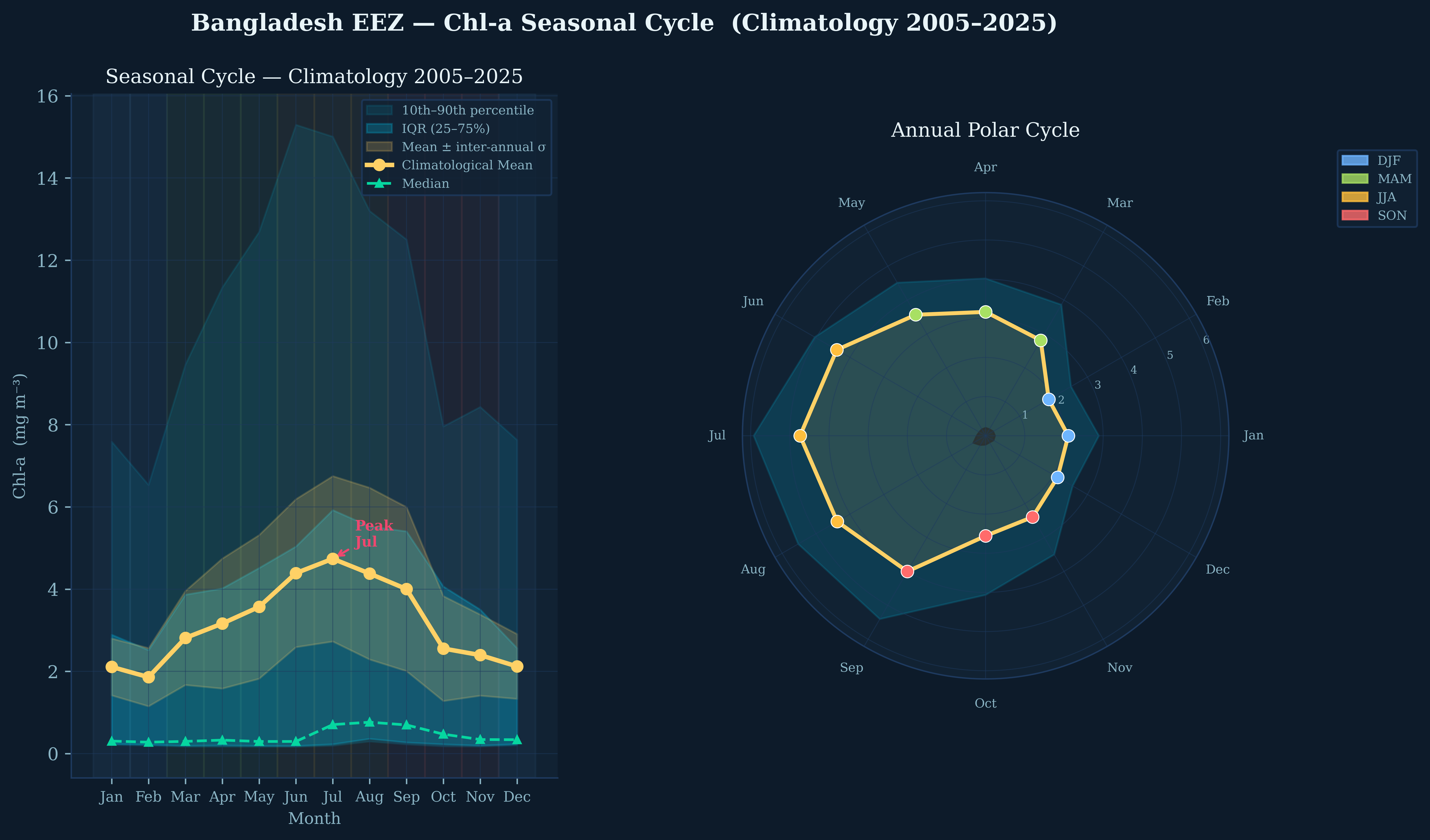
Annual Chlorophyll Cycle & Uncertainty

The climatological mean (gold line) reveals a pronounced unimodal cycle with minimum Chl-a in February (~1.9 mg/m³) and peak concentration in July (~4.7 mg/m³). The wide inter-annual standard deviation (gold shaded area) and 10th-90th percentile bands (cyan) indicate substantial year-to-year variability, particularly during the summer monsoon when river discharge is most variable.

💡 Key Insight: The polar plot reveals the asymmetric nature of the annual cycle—rapid intensification during March-June (MAM/JJA transition) followed by gradual decline through autumn, reflecting the abrupt onset of the South Asian monsoon.

❄️

DJF

Dec · Jan · Feb

2.0

mg/m³ mean

🌱

MAM

Mar · Apr · May

3.2

mg/m³ mean

☀️

JJA

Jun · Jul · Aug

4.5

mg/m³ mean

🍂

SON

Sep · Oct · Nov

3.0

mg/m³ mean

02

Where the Green Meets the Blue

The Ganges-Brahmaputra-Meghna delta creates a persistent north-south gradient, with coastal waters 10× more productive than offshore areas.

Monthly Climatological Mean Chl-a (2005–2025)

Twelve monthly composites reveal the progressive southward expansion of high-Chl-a waters during the monsoon. January-February shows minimal spatial extent of elevated Chl-a, confined to the immediate coastal zone. By July-August, the nutrient-rich plume extends far offshore, creating a broad productivity maximum centered at ~21.5°N. The logarithmic color scale (0.1–15 mg/m³) captures both the oligotrophic offshore waters and eutrophic nearshore zones.

🗺️ Spatial Pattern: The 4 mg/m³ contour (light green) advances ~150 km offshore between March and July, then retreats rapidly by October. This "productivity front" tracks the seasonal migration of the river plume and associated nutrient delivery.

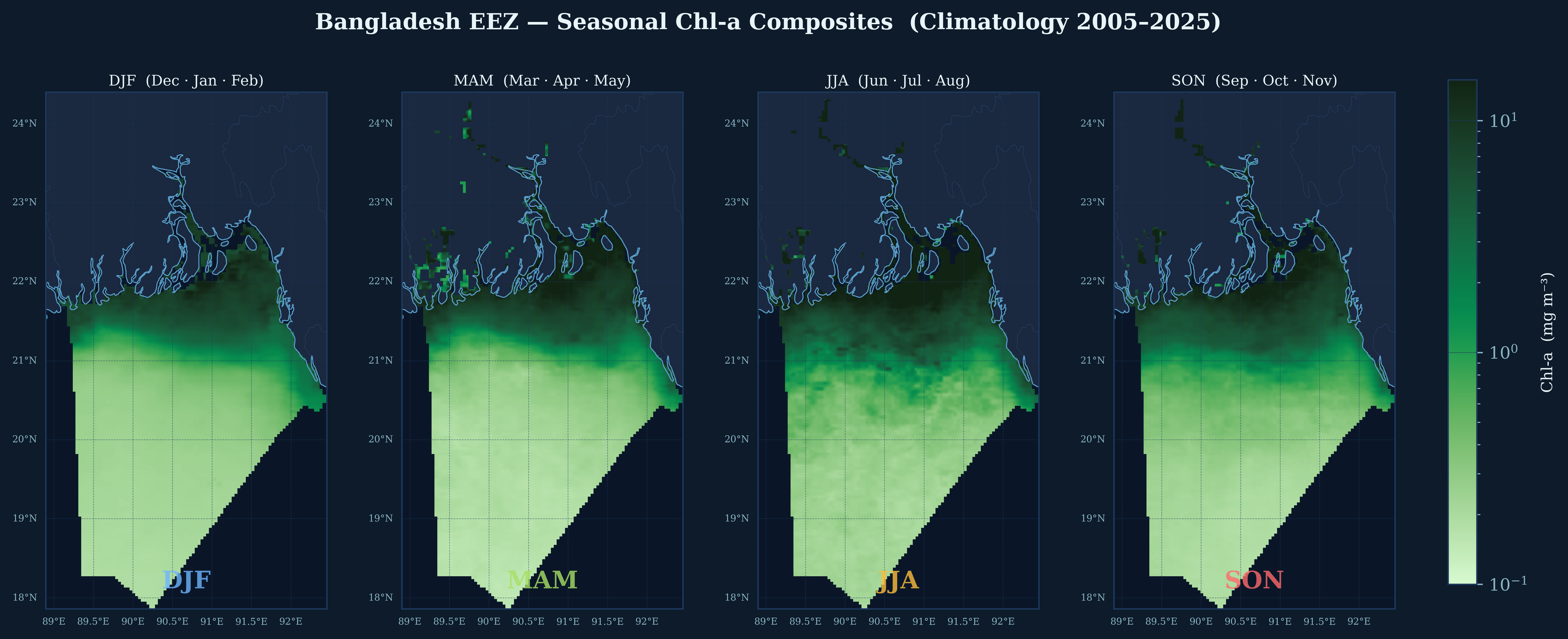
Seasonal Synthesis

Aggregating by meteorological seasons clarifies the four distinct oceanographic regimes. DJF represents the "oceanic" phase with minimal terrestrial influence. MAM shows the spring transition with developing coastal blooms. JJA captures the full monsoon impact with maximum spatial extent and concentration. SON represents the decay phase with patchy, retreating high-Chl-a features.

03

The Unstable Zone

Not all waters behave predictably. A critical band at 21°N exhibits extreme inter-annual variability, where Chl-a can vary by 100% or more between years.

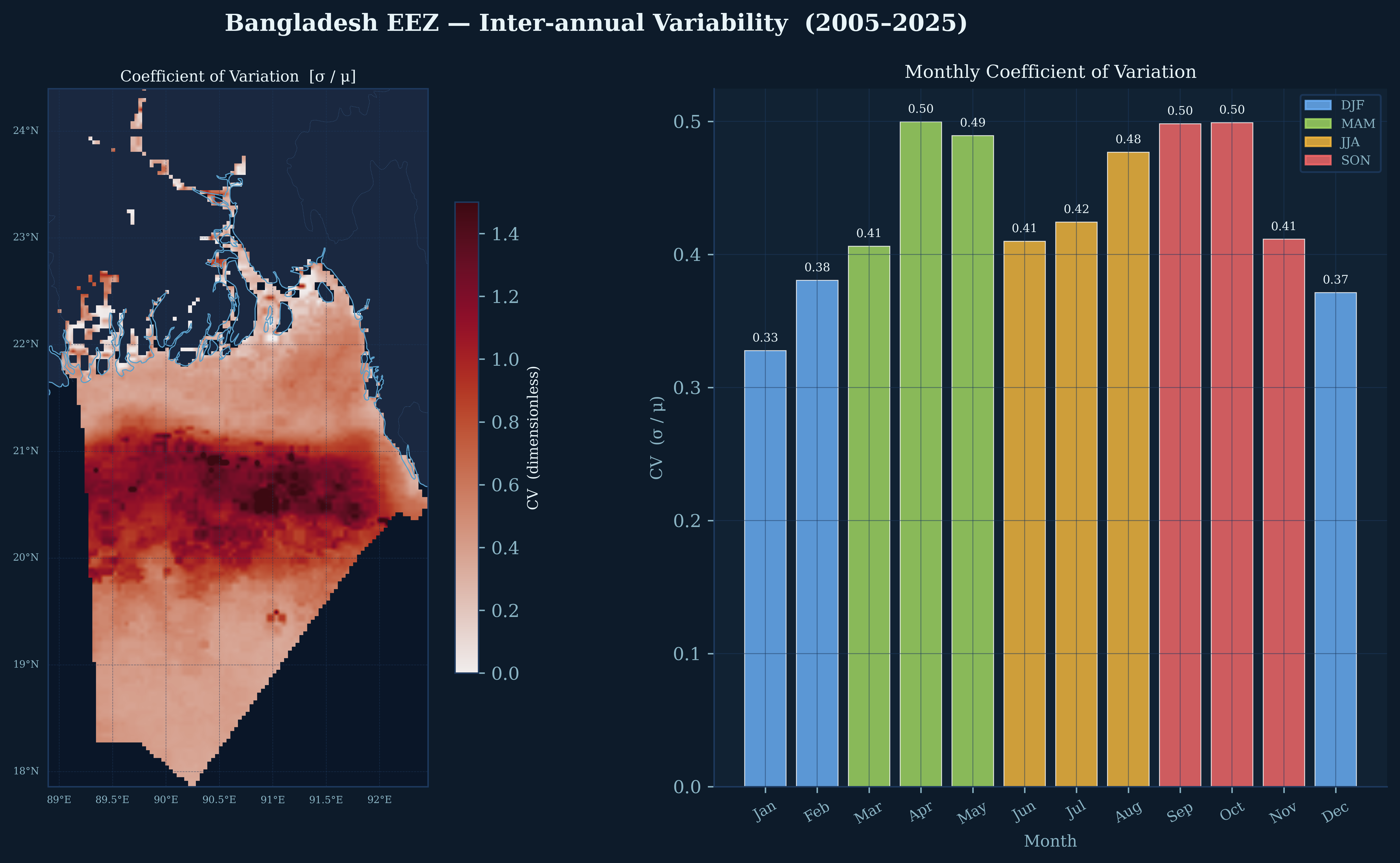
Coefficient of Variability

The spatial CV map (left) reveals a striking zonal band of extreme variability (CV > 1.0, dark red) centered at ~21°N. This corresponds to the transition zone between the stable, river-dominated northern waters and the stable, oceanic southern waters. The monthly CV bar chart (right) shows highest relative variability during the monsoon months (May-October, CV ~0.48–0.50).

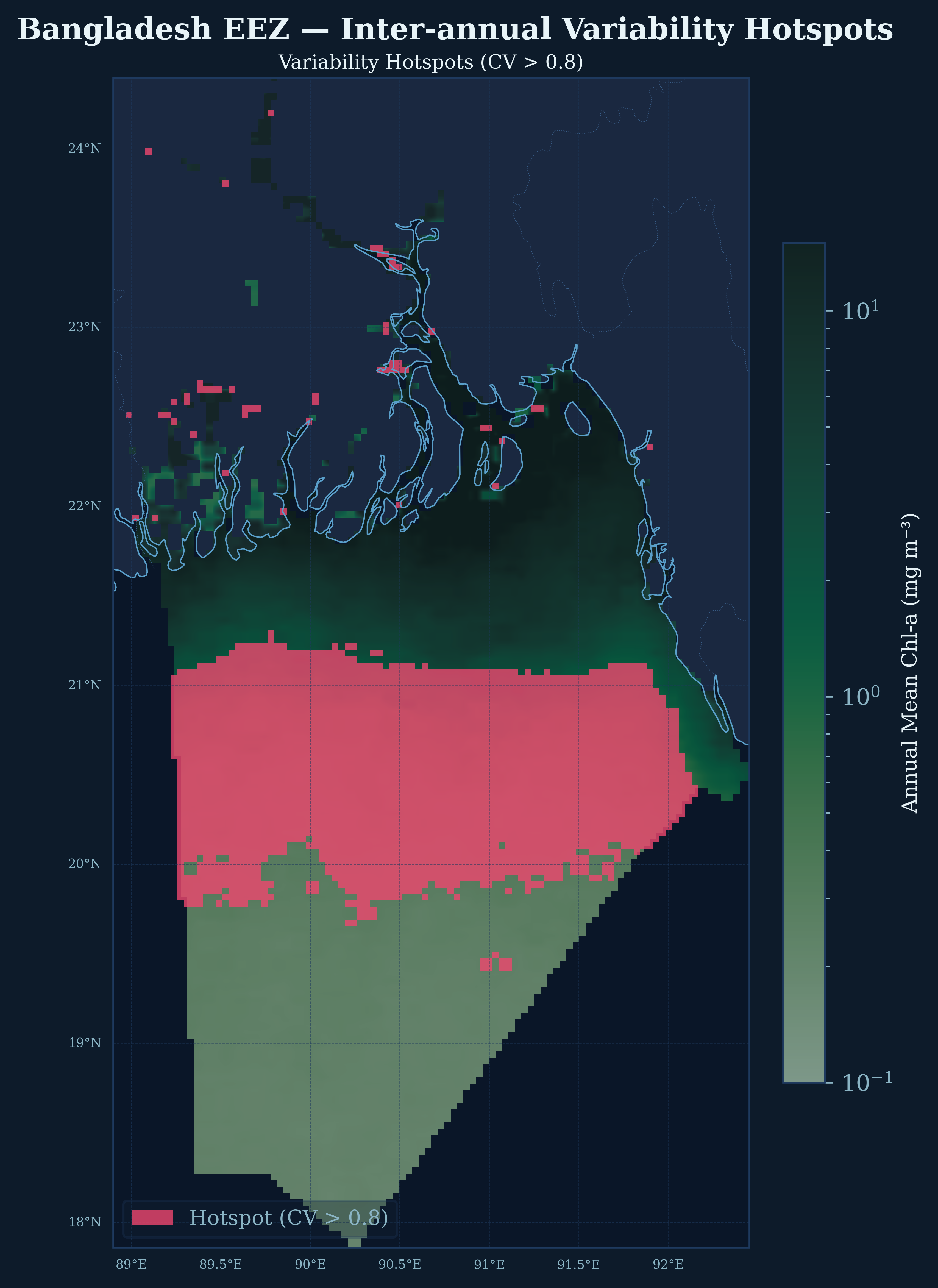
Variability Hotspots (CV > 0.8)

The 21°N band dominates the hotspot map (red overlay), indicating this is the most unpredictable region for phytoplankton biomass. Smaller coastal hotspots near the delta mouths suggest localized processes (tidal mixing, estuarine outflow) create additional uncertainty. These zones require cautious interpretation for fisheries forecasting.

Monthly Inter-annual Standard Deviation

The 12 monthly maps of inter-annual σ show that variability is not randomly distributed but follows the seasonal Chl-a cycle. Highest absolute variability occurs in July-August (σ ~2.0 mg/m³) in the northern coastal zone, coinciding with peak river discharge. The spatial pattern of variability closely tracks the mean Chl-a pattern, indicating that high-productivity areas are also high-variability areas.

⚠️ Management Implication: The 21°N variability hotspot coincides with major fishing grounds. The high CV (>0.8) indicates that Chl-a-based productivity indices alone are unreliable predictors of fishery potential in this zone—physical oceanographic context (river discharge, wind mixing) is essential.

04

Mean vs. Variability

A fundamental oceanographic principle emerges: where chlorophyll is high, it is also highly variable. The relationship is nearly perfect (r = 0.959).

Chl-a Variability & Trend Proxies

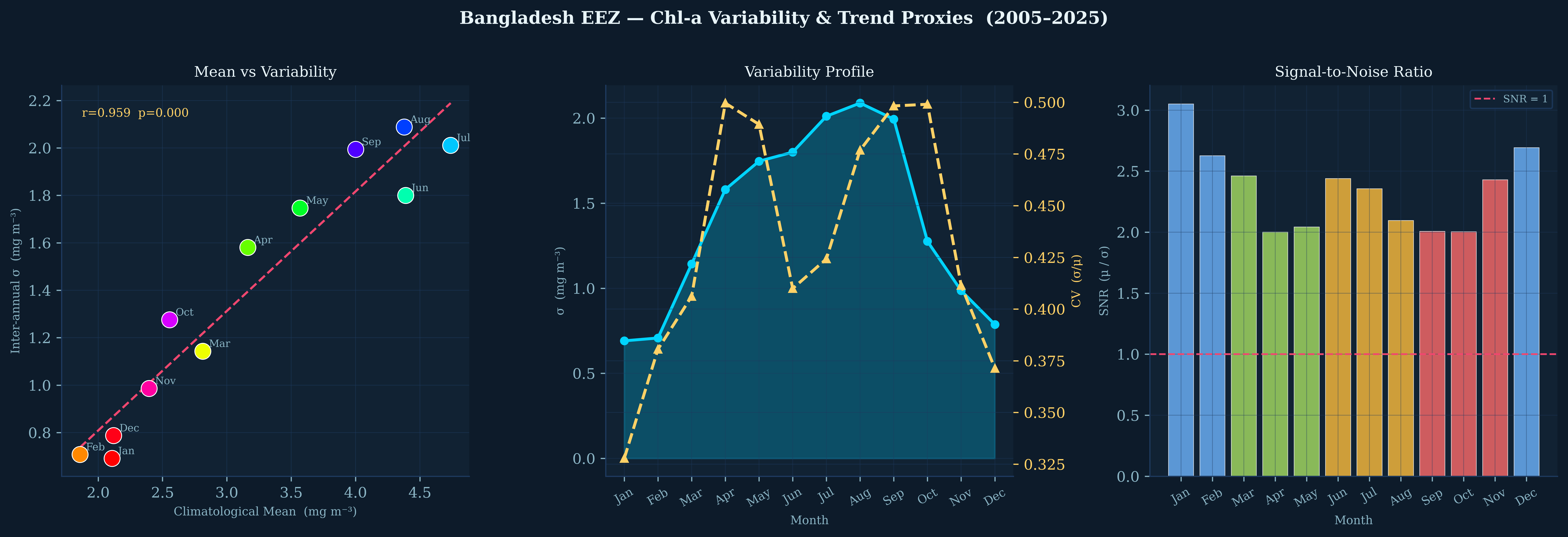
Left panel: The mean-variability scatter reveals a tight linear relationship (r=0.959, p<0.001) across all 12 months. July and August occupy the high-high quadrant, while January-February cluster in the low-low quadrant. This "Taylor's law" behavior suggests multiplicative noise processes dominate the Chl-a variability.

Center panel: The variability profile shows absolute σ (cyan) peaking in July-August, while the coefficient of variation (CV, gold dashed) shows a bimodal pattern with peaks in April-May and September-October—suggesting transition periods have highest relative unpredictability.

Right panel: Signal-to-noise ratio (μ/σ) is highest in winter months (SNR > 2.5), indicating most reliable Chl-a signals when planning research cruises or validation campaigns.

Chl-a Distribution Characteristics

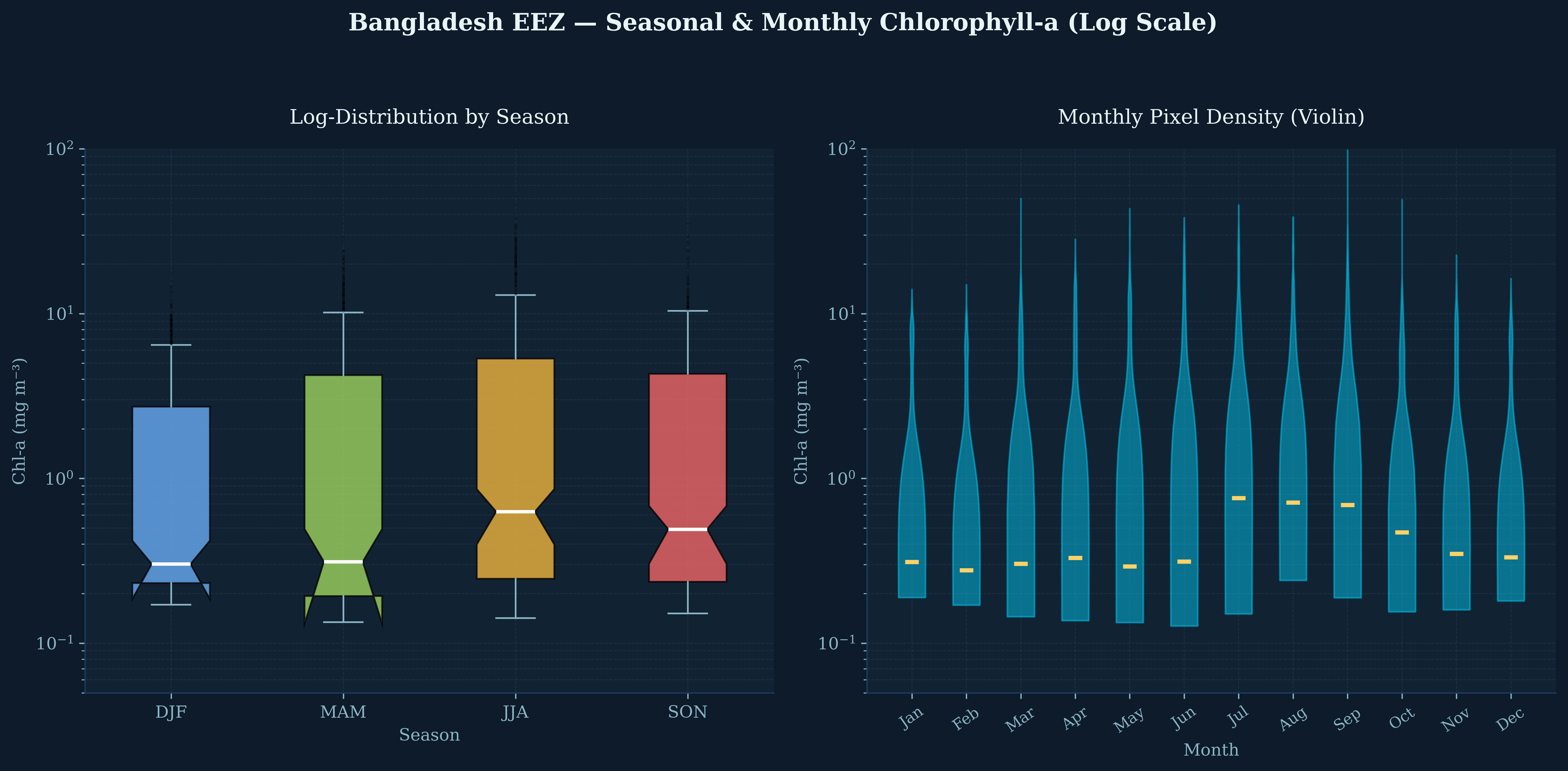
Log-transformed boxplots (left) reveal strong positive skew in all seasons, with JJA showing the widest spread (highest productivity extremes). The violin plots (right) show monthly pixel distributions are consistently log-normal, with median values (gold bars) tracking the seasonal cycle. The long upper tails indicate persistent "bloom patches"—localized high-productivity features that may represent frontal convergences or eddy-trapped nutrients.

05

Anomaly Patterns

Standardized departures from the 20-year mean reveal which months consistently deviate from "normal"—and where the Bay of Bengal is most unpredictable.

Monthly Z-score Anomaly Maps (|z| > 1.5σ flagged)

January through May show systematic negative anomalies (blue/cyan), indicating these months are consistently less productive than the annual average. June through October show positive anomalies (red/orange), with July exhibiting the strongest domain-averaged positive departure (+296,509σ in the integrated anomaly metric). The flagged pixels (|z| > 1.5σ) concentrate in the northern coastal zone, particularly around the Sundarbans region.

🔍 Anomaly Structure: The spatial pattern of anomalies is remarkably consistent across years—suggesting that "anomalous" months are actually the climatological norm, and the true anomalies are years that deviate from this seasonal expectation (e.g., failed monsoons, extreme discharge events).

Anomaly Detection & Frequency Analysis

Top row: The fraction of months exceeding annual mean (left) shows ~60% of summer months are "above average" in the northern half of the EEZ. Extreme frequency map (center) identifies the 21–22°N coastal band as experiencing |z| > 1.5σ deviations in 40–60% of years. The maximum |z| map (right) reveals localized "super-anomalies" exceeding 3σ near the delta mouths.

Bottom left: Domain-averaged monthly anomaly signature confirms the bipolar nature of the annual cycle—strong negative anomalies in winter (Jan: -194,702σ), strong positive in summer (Jul: +296,509σ). Bottom right: The heatmap shows percentage of pixels exceeding Z-score thresholds; winter months have 12–15% of domain < -1σ, while summer months have minimal extreme negative deviations.

06

Latitude as Destiny

Zonal averages reveal how the seasonal anomaly signal propagates from north to south, with distinct latitudinal "regimes" responding differently to monsoon forcing.

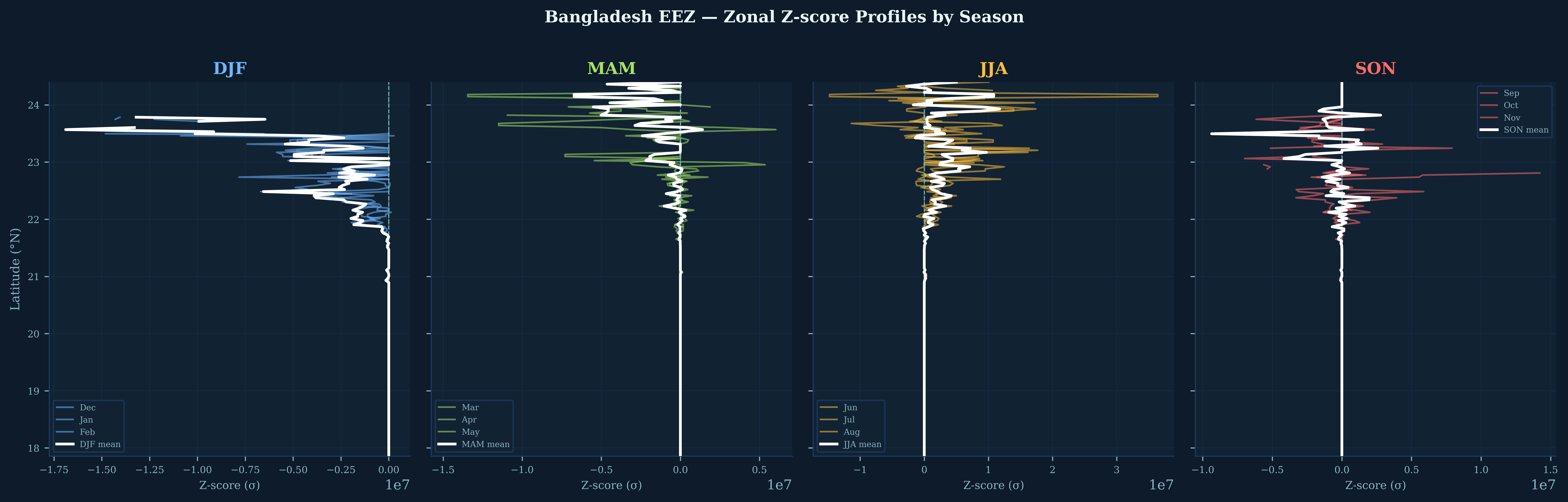
Zonal Z-score Profiles by Season

These latitude-vs-anomaly profiles reveal the vertical structure of seasonal departures. DJF (blue): Consistent negative anomalies throughout, strongest at 22–23°N. MAM (green): Transition state with near-zero anomalies at most latitudes. JJA (gold): Strong positive anomalies concentrated at 21–22°N, the core of the river plume influence. SON (red): Declining but still positive anomalies in the north, near-zero in the south.

📊 Latitudinal Regimes: Three distinct zones emerge: (1) Northern zone (22–24°N): High amplitude, river-dominated, winter-negative/summer-positive; (2) Central zone (20–22°N): Maximum variability, transition dynamics; (3) Southern zone (18–20°N): Low amplitude, oceanic, weak seasonal signal.

07

Methodology

Transparent, reproducible satellite oceanography using open data and cloud computing.

🔬 Data Processing Pipeline

All analysis conducted in Google Earth Engine with Python visualization. Code available for peer review and replication.

1

Data Source

Copernicus Marine Service Ocean Color (V6), 4km resolution, 2005–2025

2

Quality Control

Masked for nobs ≥ 1, Chl-a > 0 and < 100 mg/m³, EEZ boundary clip

3

Climatology

Monthly means across 20 years, inter-annual σ, pixel-wise CV calculation

4

Analysis

Z-score anomalies, signal-to-noise ratios, hotspot detection (CV > 0.8)

Key Metrics Defined

Climatological Mean (μ): 20-year average for each calendar month
Inter-annual σ: Standard deviation across years for each month
CV (Coefficient of Variation): σ/μ, dimensionless variability index
Z-score: (X − μ) / σ, standardized anomaly metric
SNR: μ/σ, signal-to-noise ratio for data reliability

Limitations & Caveats

Satellite Chl-a is a surface proxy; subsurface chlorophyll maxima not captured
High-turbidity coastal waters may have algorithm errors (occasional >10 mg/m³ outliers)
20-year record includes sensor changes (MERIS to OLCI transition in 2016)
No in-situ validation—patterns are consistent with literature but absolute values unvalidated